The ETF Complete model closed the week down -5.8% compared to the SPY which closed down -2.0%.

After a solid close to last week on the heels of a strong Jobs report and GDP report earlier in the month, markets dropped over the continual drip of negative news reports about the trade negotiations with China, though they closed well off their lowest levels.

Stay tuned for the daily updates and log into the website to see holdings and additional performance data.

This Week's Strategy Lesson: Measuring A Model (Part 3)

We continue this series looking at different common measures of risk. This week we will look at Standard Deviation and how it measures volatility in a stock or trading model.

Standard Deviation

Standard Deviation is a calculation of the dispersion of data points away from its average. It is used throughout statistics, finance, and other industries for a variety of purposes.

Standard deviation is based on a normal distribution (Bell Curve). Many things in the world are normally distributed: Height and weight in humans, rainfall in a region, animal populations, even the distribution of stars around many types of galaxies. In fact, the normal distribution was discovered through observations of nature and repeated trial experiments (like determining the probability of getting six heads in 10 coin flips).

The normal distribution is characterized by having a lot results clustered around the center with a severely steep drop-off in frequencies for extreme values. The average male height in the United States is 5’9’’. You would expect to find about 34 million men in the U.S. at that height, but the frequency drops off severely from there as you go higher. Yao Ming is 7’5’’ and fully six standard deviations higher than the average and there are only a handful of people over eight feet in all of recorded history.

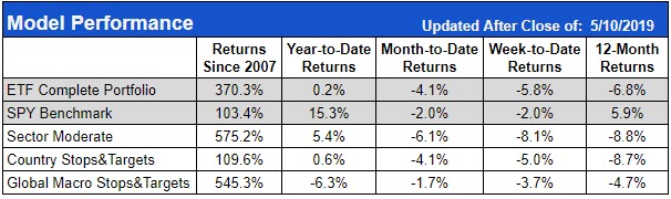
The graph above is of a normal distribution or bell curve. The blue area marked between -1 and +1 represents 68% of the total area of the curve. For normal distributions, 68% of all observations fall within +/- 1 standard deviation of the average.

If the average male height in the U.S. is 5’9’’ and the standard deviation of male height is 3 inches, then we know that 68% of all adult males in the U.S. will be between 5’6’’ and 6’0’’ (plus or minus 3 inches from the average).

Since in a normal distribution most of the observations are clustered around the center, it only takes 3 standard deviations to cover 99.7% of the observations. Going back to the height analysis, we could be rather confident that 99.7% of all adult males in the U.S. are between 5’0’’ and 6’6’’ (plus or minus 9 inches from the average).

Not everything is normally distributed. Income or wealth is not normally distributed. It tends to have “fatter tails,” meaning you see more people at the extremes than you would normally predict if it were normally distributed. Try your hardest, you will probably never run into a 50 ft. tall human in this universe or a parallel one, but you might run into someone worth $50 billion.

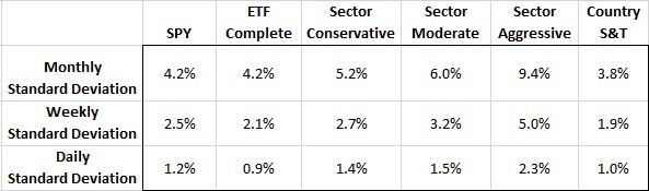
Stock returns are not strictly normally distributed, but most of the time we can use standard deviation as a good approximation. In finance, it is used for this purpose for three reasons: it works most of the time, the calculations are clean and simple and because we don’t actually know the real distribution of stock returns (and that distribution is probably not constant, fluctuating under different market conditions).

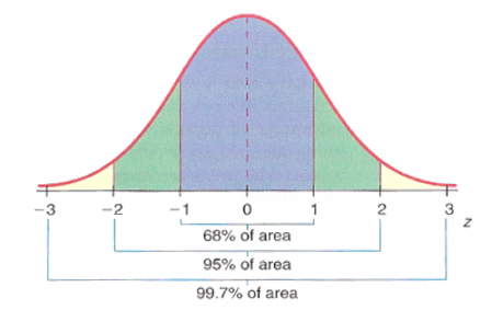
Similar to our height example, we can take stock returns (daily, weekly, monthly, etc.) and use a standard deviation calculation to determine the range and dispersion probabilities.

The table above shows the 1 standard deviation values for each of the models over daily, weekly, or monthly time frames. The 1.2% daily value for the SPY means that we can expect that 68% of the time, the SPY will close +/- 1.2% or less on a daily basis (or said another way, 32% of the time the SPY will be more volatile than +/- 1.2% on a daily basis).

As expected the weekly range is larger than the daily range and the monthly range is larger still than both.

These values give you an overall level of volatility for each of the models or instruments. Volatility can be independent of returns. You can have a low volatility strategy that does well or a high volatility strategy that does poorly. Typically, the trade-off is higher volatility to get higher returns. However, the ETF Complete has outperformed the SPY over the last 10 years while having a lower or similar overall daily and weekly volatility.

Volatility doesn’t take into account returns, but there are a few key metrics in finance that combine volatility and returns to give an overall risk-adjusted rate of return. Next week we will dive into an analysis of the Sharpe and Sortino ratios and what they tell us about our models.